Credit Availability’s Effect on Texas Rural Land Markets

Texas’ varied landscapes support diverse land uses, creating competition among potential buyers. Specifically, in growing metropolitan areas like Dallas-Fort Worth or Houston developers seeking land for urban expansion (housing, commercial, industrial) compete with buyers who have agricultural interests (farming, ranching). Another example is the competition between the energy industry (with interests that include oil and gas extraction, wind farms, solar installations) and conservation efforts aimed at preserving natural landscapes, wildlife habitats, and recreational areas.

Land-use patterns in Texas are numerous, such as cropland production, livestock, residential and recreational activities, and timber production. Such variety influences pricing and generates different income. Thus, non-agriculture factors play an important role in land sales. 

This report analyzes variations in Texas rural land values by focusing on non-agricultural factors, particularly those related to credit availability.

Background

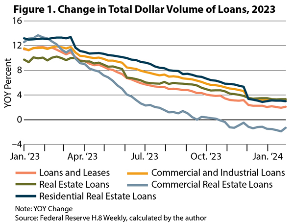
From March 2022 to July 2023, the Federal Reserve (Fed) raised the short-term federal fund rate 11 times to combat inflation. In response, banks increased their credit standards and constrained loan offers. This phenomenon is called credit tightening. As indicated by the Fed survey, loan total dollar volume decreased over the past year (Figure 1).

Market participants are less willing to take on positions under such shrinking credit conditions. This issue also affects land markets. On the one hand, potential buyers who often rely on borrowed funds to finance their investments or trading activities may choose to reduce their limit or exposure under shrinking credit conditions. On the other hand, landowners who struggle to meet the new payment and loan-to-value requirements must sell properties in a distressed situation. That causes asset prices to be even lower, and lenders become more risk-averse. Limited credit access can pose challenges to land investments and farm productivity. Over the last century, land prices have experienced three major boom-and-bust cycles that are associated with the U.S. farm business sector. The one that gains the most attention in recent studies is the 1971-85 cycle.

In the early 1970s, because of an increase in exports and crop prices triggered by a trade agreement with the Soviet Union, net farm income almost doubled in one year. Higher income encouraged farmers to expand operations. This increased activity in land markets within associated increases in transactions and prices received. However, at the onset of the ’80s, the Soviet Union’s grain embargo and a strong valuation of the dollar depressed both farm export and crop prices. Farmers were unable to generate revenue to cover the debts created in the boom period. The farming sector faced financial difficulties and began to contract further, leading to one of the greatest recessions of the agricultural economy during the late 1980s. As a result, land prices experienced a corresponding bust.

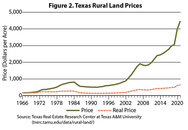
Recent record increases in rural land prices from 2000 to 2020 (Figure 2) raise concerns about the overall stability of the land market as well as the agricultural economy. The question now is, if the market begins to contract due to credit availability, will another bust come?

To explore the effect of credit availability on the state’s rural land market, this report introduces credit availability variables in a land valuation model, improving the characteristic profile (important land market influencers) of the Texas rural land market. Both county-level variation across multiple time periods and spatial contribution to the price variability measured by a spatial weighted matrix are considered. The objectives are to (1) identify credit availability effect on Texas rural land market prices; (2) identify other characteristics that determine Texas rural land market prices and determine marginal contribution of each characteristic to rural land prices; and (3) develop a characteristic profile of determinants of Texas land values that can be used by practitioners in land transactions.

Past literature has noticed the importance of such variables. For example, Sant’Anna et al.¹ fixed effect regression of counties in the Kansas City and Minneapolis Federal Reserve Districts by controlling land value determinants, credit availability factors, and county and macroeconomic factors such as unemployment rate, debt-to-income ratio, and annual population growth rate. They built an index of increased credit availability (a function of available funds, repayment rates, and collateral requirements) using Federal Reserve and Federal Deposit Insurance Corporation (FDIC) data. They found that if credit availability index goes up by 0.1, transitioning from an environment where credit availability remains the same or decreases, land price will rise about 1.96 percent or 1.64 percent depending on the index used.

Data and Model

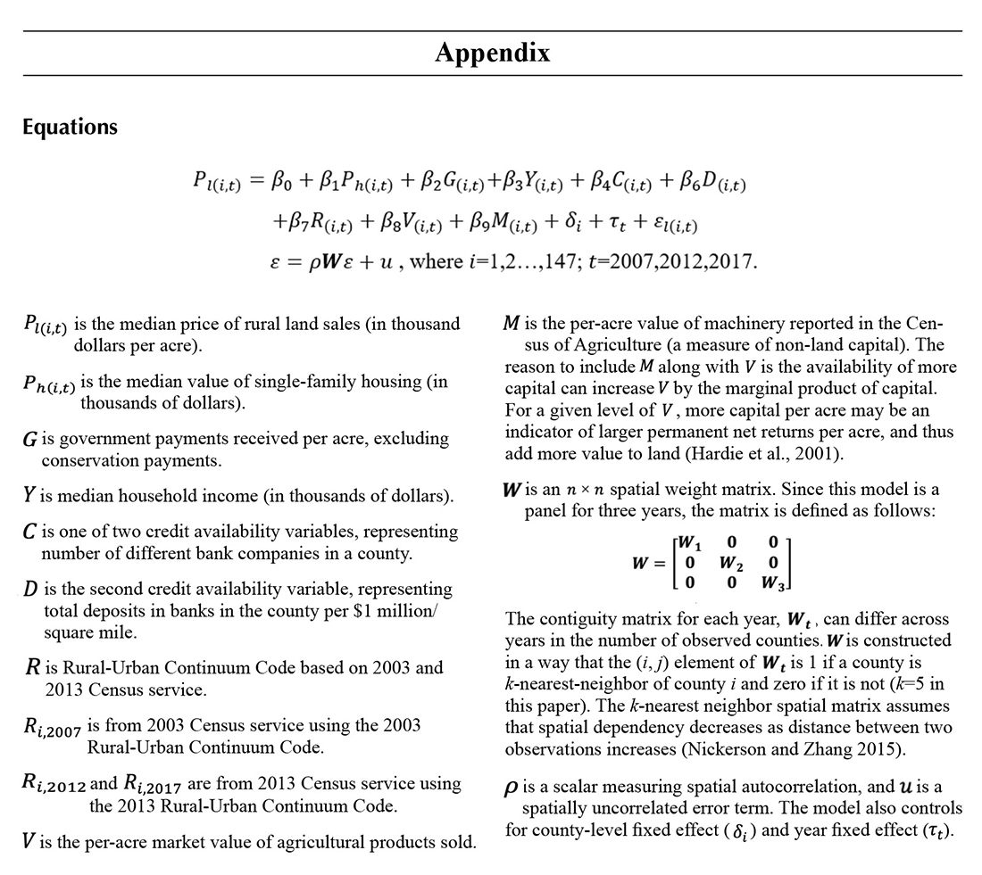
The Texas Real Estate Research Center (TRERC) at Texas A&M University collects vast amounts of the state’s land transactional data from a network of corresponding market observers, creating an excellent laboratory for studying land value determinants. Sales data includes price per acre, size of tract per sale, financing condition, total land values, previous land use, etc. This rural land database includes all reported sales not involved in urban-style developments, greater than regional minimum acreages ranging from 45 to 500 acres, and with prices less than $30,000 per acre. This study uses a county-level panel data set for the years 2007, 2012, and 2017 (Table 1). Although specific disaggregated level land parcels would provide a larger and more varied database, there is a lack of data for most key variables for such parcels, notably agricultural return data and the value of land in alternative residential use. As a result, 147 of Texas’ 254 counties are selected without missing values to construct a balanced panel.

The dependent variable, sale price per acre, is the median price of the county’s annual transaction sales data in each of the three periods. Housing value is also obtained from TRERC’s housing activity database that generates listing close price from over 50 Multiple Listing Service systems in Texas. (For more discussion on housing data, see TRERC’s website at trerc.tamu.edu/ data/housing-activity/.)

Following a study done by Rajan and Ramcharan² (2015), credit availability variables in this study include number of banks (representing more competition for depositor funds and greater credit supply) and total deposited in banks (as proxy for liquidity and lending capacity). Data are collected from the FDIC Summary of Deposits.

Returns to agricultural production (proxied by market value of agricultural products and machinery costs) and government payments are obtained from the Census of Agriculture (quickstats.nass.usda.gov/). The three monetary variables are divided by the total land in farms in each respective county, such that values are in dollars per acre.

Rural-urban continuum codes published by the United States Department of Agriculture (USDA) Economic Research Service (ers.usda.gov/data-products/ruralurban-continuum-codes/) are used to distinguish metropolitan from rural counties by population size of their metro area and degree of urbanization and adjacency to a metro area. The value ranges between one and nine and measures the urbaneness/ruralness of a county. The lower the number, the more urban the county. Both 2003’s and 2013’s codes are applied to the three-year-period data to capture a county’s possible population movement change.

The strategy in this study is to combine both agriculture and non-agriculture variables discussed earlier and apply them to a hedonic model setting. In a hedonic model, the land value can be approximated by a set of related attributes. As a result, land value is considered as a differentiated product with a combination of agricultural and non-agricultural characteristics, and each characteristic is valued by its implicit price. In this county-level study, measurement errors may occur if spatial effects on land prices do not correspond to counties as units of observation. To address the potential spatial correlation problem, this study incorporates a spatial error term into the hedonic model to control the spatial dependence. Equation details can be found in the appendix.  

Results 

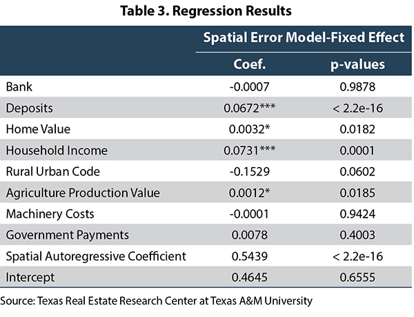
The unit of total deposits is $1 million per square mile, and each additional $1 million increase in deposits implies a $67.2-per-acre increase in land price. This suggests increases in credit availability positively but minimally impact land values (Table 2). A possible explanation could be that when banks have high availability of funds, they will grant more loans to land participants and increase the credit supply. As a result, the increase of liquidity can put upward pressure on land prices.

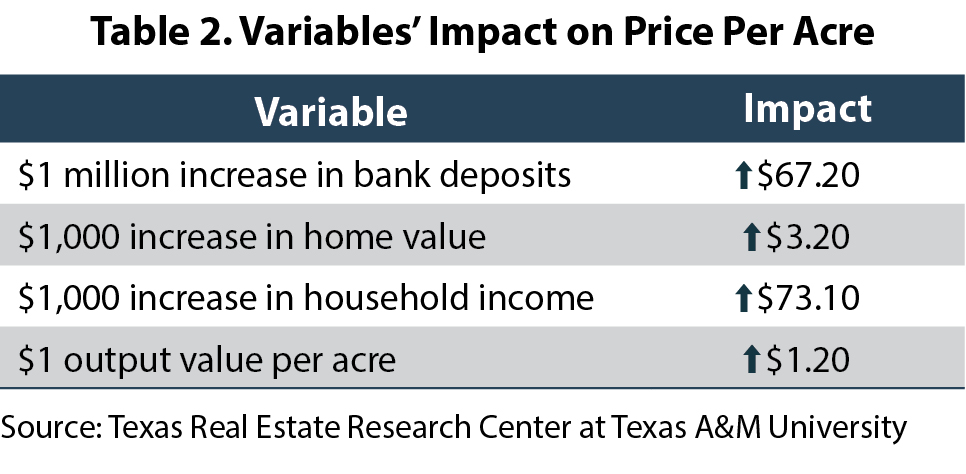
The unit of measurement for rural land price is in thousands of dollars per acre. The single-family home price is also in thousands of dollars. Thus, the coefficient of 0.0032 (Figure 3) for home value indicates that a $1,000 increase in housing price generates a $3.20 per acre increase in the price of rural land when other things are equal. This minor housing market effect is expected because there are more rural land sales than urban land sales in TRERC’s database. In other words, urban influence of transition to urban usage is smaller in rural land markets than that in urban rural fringe. The coefficient of 0.0731 means a $1,000 increase in median household income is associated with a $73.10-per-acre increase in land value. The indicated greater purchasing power supports land prices. The rural-urban continuum code, which represents one neighborhood characteristic, has a negative effect (-0.1529) on rural land values. The larger the code, the more rural the county. The further from metropolitan cities (based on population classification), the less the demand for commercial land. The coefficient of per-acre market value of agricultural products sold is significant. It means a $1.2 land price increase for a $1 increase in output value per acre. This result shows that agricultural factors still contribute to Texas rural land market’s values.

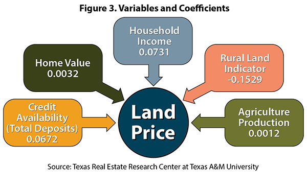
Table 3 (see Appendix) shows the estimation results of the spatial-error panel regression model in a hedonic setting under fixed effects assumption, controlling for both county and time effects. The significance of the spatial autoregressive coefficient, which is below 1 percent significant level, confirms the existence of spatial correlation between counties. It also confirms the land value dependence among neighboring counties. This dependency is not captured by explanatory variables in the model. Therefore, spatial clustering of residuals exists in model, demonstrating the importance of the effect of neighboring counties.

Conclusion

In all, this study finds several non-agricultural factors that drive Texas rural land values, including credit availability, which has a positive effect. This conclusion has also been discussed more in recent land value studies. Lenders can assess and mitigate loan risks and better manage their investment portfolios if they are aware of these positive impacts and the potential change in land values.

The study also examines the positive effect of an increase in median household income on land value. This is consistent with TRERC’s earlier research findings, which indicate the growing association between personal income and land prices. The return from agriculture also plays a critical role as the bottom line of support in most rural land values. Therefore, a characteristic profile of determinants of land values of Texas rural land markets has been built that includes credit availability, housing values, ruralness/ urbaneness, household income, and variables related to agriculture return according to the empirical analysis results.

References

¹ Sant’Anna, A.C., C. Cowley, and A.L. Katchova. 2021. “Examining the Relationship between Land Values and Credit Availability.” Journal of Applied Agricultural Economics 53(2):209–228.

² Rajan, R. and Ramcharan, R., 2015. “The Anatomy of a Credit Crisis: The Boom and Bust in Farm Land Prices in the United States in the 1920s.” American Economic Review 105(4), pp.1439-1477.

References

1 Sant’Anna, A.C., C. Cowley, and A.L. Katchova. 2021. “Examining the Relationship between Land Values and Credit Availability.” Journal of Applied Agricultural Economics 53(2):209–228.
2 Rajan, R. and Ramcharan, R., 2015. “The Anatomy of a Credit Crisis: The Boom and Bust in Farm Land Prices in the United States in the 1920s.” American Economic Review 105(4), pp.1439-1477.
You might also like
Land Occupier’s Liability Guide
This guide provides an introduction to land occupier’s liability in Texas. It gives a basic understanding of liability concepts and the potential pitfalls for owners and occupiers of land. This guide does not cover every situation for which a land occupier might have liability, nor does it cover every point of law that might be applicable.
TG Magazine
Check out the latest issue of our flagship publication.