Life After Economic Data Revision

In the first four months of each year, the U.S. Bureau of Labor Statistics (BLS) revises its previously published employment data. Not surprisingly, the Real Estate Center receives many emails and phone calls after these revisions from people who use the employment data from the Center’s publications. This article responds to some recent queries.

Economic Data Revisions

Users of economic indicators confront three major data problems: delays and lags in the release of the current period data, repeated data revisions and data errors. While users need timely and accurate data, in the real world it takes time to collect, organize and disseminate economic data, and to improve data accuracy.

For instance, the Bureau of Economic Analysis (BEA) of the U.S. Department of Commerce releases an “advance” figure for the U.S. gross domestic product (GDP) one month after the end of the quarter with a caveat that the “advance estimate released today is based on source data that are incomplete or subject to further revision by the source agency.” One month later the BEA releases a revised “preliminary” figure based on more collected information and survey evidence. Two months later the “final” estimates of quarterly GDP data based on more collected information are released.

As households and firms file their tax returns, the BEA uses more accurate income and employment data for estimating national income and product accounts (NIPA), and every July NIPA estimates for the previous four quarters are revised. The revision is repeated for the next two years. Then, at five-year intervals, the BEA releases its “Comprehensive Revision” of the NIPA data, mostly based on the analysis of tax returns rather than on survey samples and models. From time to time, when the BEA changes its methodology and develops more exact estimation methods, it revises NIPA data back to 1929. The bottom line is that data (including employment data) are almost continually updated.

Employment time series data are the most widely watched economic indicators for gauging the direction of state and local economies. They are compiled on a monthly basis by the BLS and local workforce commissions, such as the Texas Workforce Commission (TWC). The BLS releases its “first preliminary” estimates of employment, hours and earnings through its Current Employment Statistics (CES) survey program each month approximately three weeks after the reference period. These estimates are revised one month later in the “second preliminary” report. The sample-based estimates are again revised two months after the initial release.

Historical labor force and employment data for the United States and state and local areas are revised annually in the first four months of each year. The revisions include nonagricultural wage and salary employment for the past two years. For instance, revisions of Texas employment data for 2012 and 2013 are published in the first four months of 2014. The annual benchmark revisions may update employment data as far back as 1990 on the websites of the BLS or TWC. From May, the BLS revises only the previous month’s employment data each month and leaves the historical data in peace until the next January.

Repeated data revisions by the BEA, BLS and other agencies mean there is no such thing as “final” or “actual” economic indicators; rather, all economic indicators are continually revised versions of older data.

We all know that to err is human, but it is important that data errors are reported as soon as detected. The BLS has a website (www.bls.gov/bls/erratabydate.htm) that publishes its errors and corrections. In 2013, the BLS detected and corrected 49 data processing errors. Other data-supplying agencies, such as the BEA, have error-reporting policies on their websites.

Learning from Repeated Data Revisions

Repeated data revisions by the BEA and other agencies, while necessary to produce more accurate data, have made it more difficult for market participants to make business decisions, for economists to make forecasts, for macroeconomic policy makers to implement fiscal and monetary policies, and for candidates in the midst of political campaigns.

For market participants and forecasters of economic indicators, repeated data revisions mean uncertainty about past, current and future data. To deal with data uncertainty, in recent years a number of economists in the United States and other countries have compiled vintage datasets or real-time datasets for economic indicators and have developed methods for analyzing the impact of data revisions on macroeconomic policy. In the past, previous vintages or versions of data were normally superseded by new data as more accurate data became available. But now, a number of agencies retain all past vintages of data to be used for economic research. In the United States, the St. Louis Fed offers ALFRED (ArchivaL Federal Reserve Economic Data) allowing users to retrieve vintage versions of economic data that were available on specific dates in history.

Data delays and revisions have been important factors in diminishing expectations about the government’s ability to fine-tune the economy. After John Maynard Keynes published The General Theory of Employment, Interest and Money (1936), governments of the United States and some other developed countries influenced by Keynesian economics adopted a number of macroeconomic policies, known as counter-cyclical policies, for controlling the pace of output and employment growth rates in their economies. According to adherents of Keynesian counter-cyclical policies, the government may be able to help the economy come out of a recession through a combination of fiscal and monetary policies such as increasing government expenditures and decreasing interest rates. Conversely, government can put the brakes on a fast-growing economy by decreasing government expenditures and increasing interest rates.

Implementation of these policies in the 1970s failed to attain their targets, leading to stagflation, an economic situation characterized by a slow economic growth rate coupled with high inflation rates. Macroeconomic policy makers and economists noted that it takes several months to know whether an economy is in recession because of data delays. It takes more than six months for the full impact of macroeconomic policies on the economy to be realized. By that time, the economy may recover by its own dynamics, rendering macroeconomic policies detrimental.

Political campaigners relying on economic indicators need to be wary of data revisions during election campaigns. For instance, in the 2014 Ohio governor’s election race, candidate Ed FitzGerald (D) claimed that Ohio ranked 45th among states in job creation in 2013. A week later, revised figures showed that Ohio was 26th, a figure used by his rival to prove that the Ohio job market was not as bad as portrayed by his opponent.

Trends May Be Your Friends

Looking at various vintages of time series economic indicators, we find two rays of hope in data revisions. First, aggregate or total economic indicators, such as total employment growth rates for Texas, tend to be revised less substantially than their components. For instance, Texas’ total employment growth rate tends to be revised less substantially than employment growth rates for the state’s industries. Second, although the absolute values of economic indicators may change in data revisions, the underlying trends in growth rates normally do not alter to a significant degree. The lesser volatility of underlying trends in growth rates of most major economic indicators imply that market participants and forecasters may be able to grasp the directions of economic changes by focusing attention on the underlying trends in time series data and by employing statistical methods that extract longer-term economic trends from those data.

Because of the importance of the underlying trends in data, the Real Estate Center at Texas A&M University publishes trends in data over time in addition to snapshot comparisons of employment growth rates for the state’s industries and metropolitan areas.

Employment Data Revisions, 2014

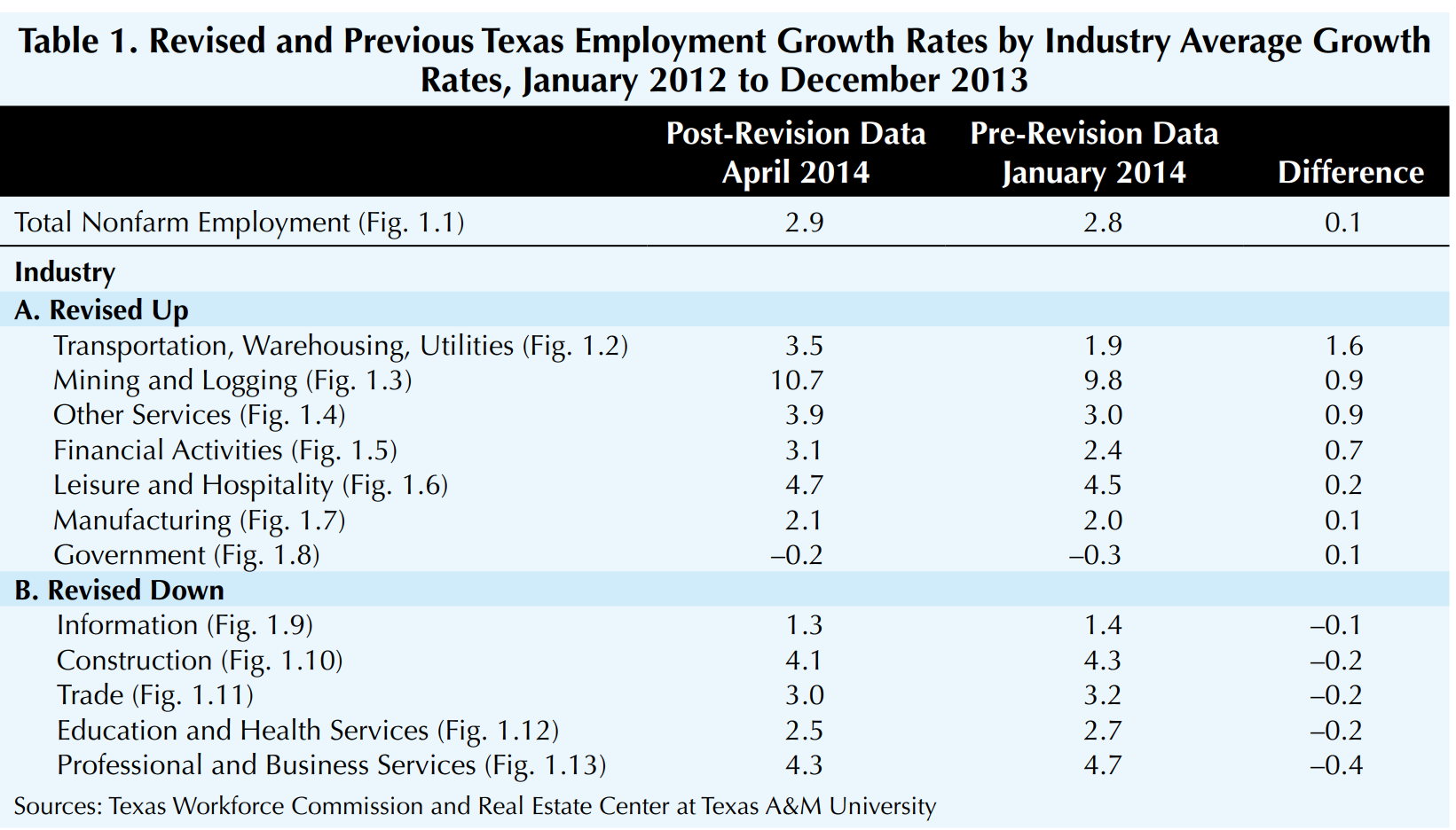
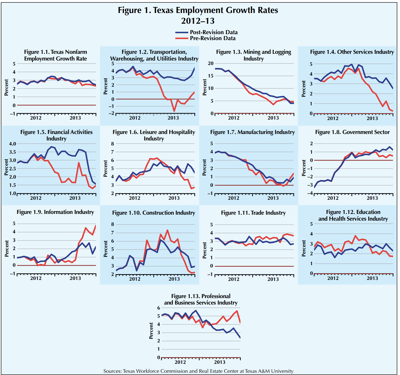
Table 1 presents the average growth rates of Texas total nonagricultural employment from January 2012 to December 2013, before and after 2014 employment data revisions, and Texas industries ranked by the size of revisions. The average growth rate of Texas nonagricultural employment from January 2012 to December 2013 was revised upward from 2.8 percent to 2.9 percent after 2014 data revisions (Table 1 and Figure 1). The underlying trend in employment growth rate in Figure 1 shows that the state economy continues to generate jobs at annual rates of close to 3 percent according to both old and revised data. However, employment growth rates for components of the state’s economy — employment growth by industry — are revised more substantially than total employment growth rates.

Six Texas industries and the state’s government sector experienced upward revisions (Table 1, Panel A) while employment growth rates in five Texas industries were revised downward (Table 1, Panel B). The state’s transportation, warehousing and utilities industry experienced the largest upward revision followed by mining and logging, other services and financial activities.

Figures 1.2 to 1.13 show trends in employment growth rates for Texas industries before and after the 2014 data revisions.

Table 2 presents Texas metropolitan areas ranked by the size of revisions in average annual employment growth rates from January 2012 to December 2013. College Station-Bryan experienced the largest upward revision, followed by San Antonio-New Braunfels, Austin-Round Rock-San Marcos, Sherman-Denison and Victoria (Table 2, Panel A). The average annual employment growth rates for the Houston-Sugar Land-Baytown and San Angelo metro areas remained unchanged in the aftermath of 2014 data revisions (Table 2, Panel B). Odessa experienced the largest downward revision followed by Beaumont-Port Arthur, Longview, Texarkana and Waco (Table 2, Panel C).

Figures 2.1 to 2.26 show trends in employment growth rates for Texas metro areas before and after the 2014 data revisions.

Dr. Anari ([email protected]) is a research economist with the Real Estate Center at Texas A&M University.